01Overview
GraphMind trains a two-layer graph convolutional network (GCN) to predict the research topic of a machine-learning paper from two sources of information: the words the paper uses and the papers it is connected to by citations. The trained model is exported to ONNX, served by a FastAPI backend, and explored through an interface that shows each prediction alongside the paper’s citation neighbourhood.
The project began from a public tutorial notebook. It was extended with a graph-exploration interface, a live re-evaluation of the exported model, an edge-ablation experiment, input validation for the API, and this write-up of its limitations.
02Problem statement
Given the Cora citation graph — 2,708 papers, 5,278 citation links, and a 1,433-dimensional bag-of-words vector for each paper — predict which of seven topics each paper belongs to. Only 140 papers have training labels. This is semi-supervised, transductive node classification: the whole graph, including the test papers’ features and links, is visible during training and inference, but their labels are not.
03Motivation
Papers that cite each other tend to share a topic. The question this project tests is concrete: how much does using that citation structure add over classifying each paper from its own words alone? Cora is small enough to inspect paper by paper, which makes it a good setting for seeing where message passing helps and where it misleads.
04System architecture
- Data — Cora from PyTorch Geometric’s Planetoid loader (public split), stored with the repository.
- Model —
GCNConv(1433→32)→ ReLU → dropout 0.5 →GCNConv(32→7); logits over seven topics. - Export — trained in PyTorch, exported to ONNX (opset 18, about 250 KB) with node features and edge indices as inputs.
- Serving — FastAPI with ONNX Runtime on CPU:
POST /predict/cora_nodefor real papers,POST /predictfor a custom graph. - Research endpoints — a thin adapter adds read-only endpoints for neighbourhoods, dataset statistics and evaluation; every prediction still comes from the same inference function.
- Interface — HTML, CSS and JavaScript with SVG graph rendering; no frontend framework.
05Technical implementation
- Training in PyTorch Geometric with Adam (learning rate 0.01) and cross-entropy on the 140 labelled papers.
- Early stopping on validation accuracy with a patience of 20 epochs; training stopped at epoch 35.
- The API validates input shapes, feature length (1,433) and node indices, returning HTTP 400/422 rather than crashing — including for edges that point to nodes that do not exist.
- The evaluation endpoint runs the exported ONNX model once over the full graph and computes accuracy, macro-F1, per-class metrics and a confusion matrix for each split.
06Dataset and preparation
| Papers (nodes) | 2,708 |
|---|---|
| Citation links (undirected) | 5,278 |
| Features per paper | 1,433 binary word indicators (mean 18 active) |
| Topics | 7 |
| Split (train / validation / test) | 140 / 500 / 1,000 |
| Node degree | median 3, mean 3.9, max 168 |
Planetoid ships only the binary word indicators, not the papers’ text or vocabulary, so the interface cannot show which words a paper contains — only how many are active.
07Model design
Each GCN layer replaces a paper’s representation with a degree-normalised average of its own and its neighbours’ representations, followed by a learned linear map. Two layers give every prediction a two-hop receptive field: a paper is informed by the papers it cites, the papers that cite it, and their neighbours. With only 140 labels, a small hidden layer (32 units) and dropout of 0.5 limit how much the model can memorise.
08Evaluation methodology
- Re-evaluation of the shipped model. The server scores the exported ONNX file — not the notebook’s in-memory model — on the public split.
- Edge ablation. The same model and features, with every citation edge replaced by a self-loop, isolates how much the predictions depend on graph structure.
- Baseline. A random forest on TF-IDF-reweighted word indicators, with no graph information, from the training notebook.
09Verified results
| Model / setting | Accuracy | Macro-F1 | Source |
|---|---|---|---|
| Two-layer GCN (shipped ONNX) | 0.792 | 0.782 | re-evaluated |
| Same GCN, citation edges removed | 0.678 | 0.661 | re-evaluated |
| Random forest, words only | 0.581 | 0.570 | notebook |
| GCN on validation (500) | 0.792 | 0.775 | re-evaluated |
| GCN on training labels (140) | 1.000 | 1.000 | overfit |
Per-topic F1 on the test split
| Topic | F1 | Test papers |
|---|---|---|
| Genetic Algorithms | 0.870 | 144 |
| Probabilistic Methods | 0.820 | 149 |
| Neural Networks | 0.809 | 319 |
| Case Based | 0.771 | 103 |
| Reinforcement Learning | 0.762 | 91 |
| Rule Learning | 0.735 | 64 |
| Theory | 0.710 | 130 |
Removing citation edges costs 11.4 accuracy points with the same weights, so the trained model relies substantially on graph structure. This is not the same as comparing against a model trained without the graph — see the limitations.
10Demonstration video
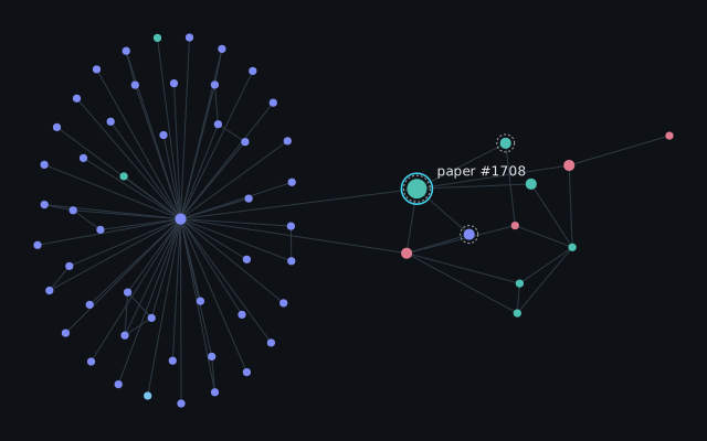
Recorded on the live deployment, 11 October 2026; no audio. Paper 1708 is classified and widened to two hops, a misclassified test paper is opened, the edge experiment is run on real Cora features, and the server-side evaluation is shown.
11Deployment and source code
- Live demo: anshaiml369.github.io/graphmind — Hugging Face Space (Docker, 2 vCPU, 16 GB). On the earlier Render free plan (512 MB, shared CPU), loading the dataset on the first evaluation request took about 49 s.
- Runtime: Python 3.11 with pinned dependencies and the CPU-only PyTorch wheel (PyTorch is used only to load the dataset).
- Source code: available on request.
12Limitations and known failure modes
- One training run, no fixed seed. No variance across seeds is reported, so the 0.792 should be read as one sample.
- Checkpointing bug. The notebook stores
model.state_dict()by reference, so the exported weights are the final-epoch (35) weights, not the best-validation weights (validation accuracy 0.792 versus a logged best of 0.812). - Overfitting. Training accuracy is 1.000 on 140 labelled papers.
- Transductive setting. Test papers’ features and links are present during training; results do not show performance on papers added later.
- The ablation is not a trained baseline. Removing edges from a model trained with them understates what a model trained without edges (for example an MLP) could achieve.
- A documentation error in the notebook. Its text says the random-forest baseline uses degree features; the code uses word features only.
13Future improvements
- Train over several seeds and report the mean and spread.
- Fix the checkpoint copy and re-export the best-validation weights.
- Add an MLP trained on the same features without the graph, and compare with GAT or GraphSAGE.
- Evaluate an inductive split in which test papers are unseen during training.